SolveItClass 9 · NCERT

NCERT Solutions · Class 9 Science Sound Waves: Characteristics and Applications

28 questions · 16 still being checked

Pause and Ponder 10.5–10.6 (part 8 of 21)

  1. Exercise 10.5

    Now, push and pull the slinky end multiple times in quick succession (The pulling and pushing of the end of the slinky is similar to the sound being produced continuously). Are a series of disturbances produced in the slinky? Do these disturbances move across the length of slinky? Does the mark on the slinky move back and forth parallel to the direction of the disturbance? Turns are closer together

    Not cross-checked

    NCERT prints no numerical answer for this exercise, so this working has not been cross-checked against the book.

    NCERT’s answer
    (ii)
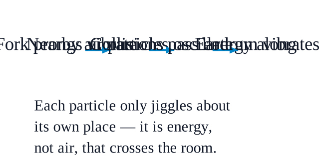
    (ii) Energy carried by sound waves.
    NCERT_Solution_Class9_Science_Ch10_PP_Q10-5
    The air particles near the fork only oscillate about their mean positions and never travel to your ear, so (i) and (iv) are wrong — there is no stream of air moving across the room.
    The fork's material stays in the fork, so (iii) is wrong.
    Sound is a form of energy: the vibrating prongs hand energy to the neighbouring air particles, whose collisions pass it on from particle to particle until it sets your eardrum vibrating.
  2. Exercise 10.6

    The variation of density of the medium for two sound waves is shown in Fig. 10.17\displaystyle 10.17 (a) and (b). Label compression and rarefaction by C and R on it. In the graph given in Fig. 10.17\displaystyle 10.17 (c) and (d), label the axes and draw the curves corresponding to Fig. 10.17\displaystyle 10.17 (a) and (b).NCERT_Question_Class9_Science_Ch10_PP_Q10-6

    Not cross-checked

    NCERT prints no numerical answer for this exercise, so this working has not been cross-checked against the book.

    Compressions (C) are the crowded regions and rarefactions (R) the thinly spread ones — mark them alternately, C R C R …, along both Fig. $\displaystyle 10.17$ (a) and (b).
    In (a) and (b): write C wherever the dots representing the particles are packed closer than average, and R wherever they are more spread out than average.
    For graphs (c) and (d): label the x-axis "Distance" and the y-axis "Density".
    Draw a horizontal dashed line across each graph for the average density — this is the level the curve oscillates about.
    On each graph draw a smooth wavy curve with a crest (maximum density) directly above every C and a trough (minimum density) directly above every R, the curve cutting the dashed line midway between them.
    Keep both graphs on the same distance scale: the strip whose C's are closer together must give the curve with crests closer together, i.e. the shorter wavelength, and the other strip the longer-wavelength curve.
    The height of a crest above the dashed line (and the depth of a trough below it) is the density amplitude — draw it the same on both unless one strip is visibly more crowded than the other.